

LEARN | Revision Module
Congratulations on making it through F4F LEARN! We hope that you have found the modules interesting and informative, and that you now feel more confident about critically appraising scientific literature.
In preparation for the final exam, we have prepared a revision module for you all. If you read over this entire module, you should be prepared for anything the exam will throw at you!
Just as a reminder, the final exam is compulsory for those who wish to take part in Phase II of F4F LEARN, in which Monash and UPSM students will collaborate on their own research projects.
As always, please post any questions, comments or suggestions in the Disqus comment feed at the bottom of the module!
Introduction to Evidence Based Clinical Practice
Asking an answerable question
Patient
Intervention
Comparison
Outcome
Remember to search databases such as the Cochrane library with a search strategy that uses the words AND (to combine different concepts) and OR (to combine synonyms). For detailed instructions, see this document.
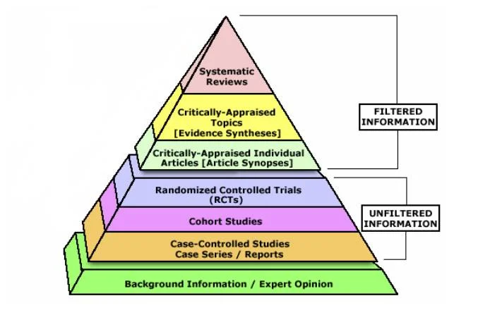
The evidence pyramid
The gold-standard single study is a randomised controlled trial (RCT), whereas the lowest tier of evidence is expert opinion. A systematic review and meta-analysis of multiple high-quality RCTs is the highest tier.
Different Types of Studies
Systematic Reviews
An overview of primary studies with a defined methodology that is reproducible. A thorough and transparent process reduces the risk of bias. A meta-analysis can be performed to provide greater statistical power than any individual study. A meta-analysis takes into account all primary studies, whether they showed statistical significance or not. A meta-analysis can, however, separately analyse good quality and bad quality studies.
Randomised Controlled Trials
Randomised: patients are assigned to either an intervention or a control group at random. The randomisation usually ensures that all characteristics (both known and unknown) are equal between intervention and control groups.
Controlled: all participants are treated the same aside from the intervention being performed (e.g. both placebo and intervention patients get the same amount of follow-up visits/observation).
Double-blinded: neither the patients nor clinicians know who is in what group.
Cohort Studies
A cohort study is observational – investigators identify a cohort of people with an exposure, and a cohort of matched controls without the exposure. They then follow these two groups, forwards in time, and see who develops an outcome. These are ideal for studies looking at prognosis, or what a particular exposure places you at risk of.
Case-Control Studies
A case-control study is also observational. Investigators identify a group of cases (people with a disease), and match them with a group of controls (people without disease). They then look backwards in time to see what they were exposed to. These are ideal for studies looking at rare diseases.
Biostatistics
Data can be classified as:
- Categorical
- Ordinal (e.g. cancer staging)
- Nominal (e.g. hair colour)
- Numerical
- Discrete (e.g. number of children in a family)
- Continuous (e.g. blood pressure)
It is possible to convert data from numerical to categorical, but not the other way around.
The p-value
The p-value essentially tells us how likely it is that the result obtained is due merely to chance. When the p-value is 0.05, the scientific community has arbitrarily decided that this means the result is statistically significant – there is only a 5% probability that the result was only due to luck.
Confidence Interval
The confidence interval is the range within which the population mean is likely to lie. This means that if the 95% confidence interval is 0.30 to 1.10, there is a 95% probability that the population mean is between these two numbers.
It is important to remember that if the confidence interval crosses a relative risk of 1 (i.e. there is no difference), then the result is not statistically significant. For the same reasons, if the confidence interval crosses an absolute risk of 0 (i.e. there is no difference), the result is not statistically significant.

Clinical Significance
The p-value and confidence interval have been discussed in terms of statistical significance. To be clinically significant, the risks and benefits of a particular intervention must be looked at together (e.g. warfarin use for stroke prevention in atrial fibrillation). A further measure of clinical significance is the number needed to treat, described below.
Measures of Treatment Effect
Relative risk (RR) and relative risk reduction (RRR)
A relative risk for harm (death) of 0.5-1 is weak, 0.125-0.5 is moderate and <0.125 is strong. A relative risk for benefit (cure) of 1-2 is weak, 2-4 is moderate and >4 is strong.

The relative risk reduction refers to 1 - RR. (e.g. for a relative risk of 0.7, the RRR is 1 - 0.3 = 0.3 = 30%).
Number needed to treat (NNT) and absolute risk reduction (ARR)
It is the number of people needed to give the intervention to in order to prevent a bad outcome or achieve a good outcome. For example, in a study where the "risk" was cure, a NNT of 5 people means that giving 5 people the tested intervention will mean that one of them is likely to be cured (on average).

External validity
External validity looks at whether the results of a trial are valid for your patient. Would they fit the inclusion and exclusion criteria or are people like them not accounted for in the trial?
Bias
- Selection bias – control and experimental groups are different at baseline, prevented using randomisation
- Performance bias – different care given depending upon group, prevented using blinding
- Attrition bias – people dropping out, controlled for using intention to treat analysis
- Detection bias – outcomes assessed in different ways, prevented by blinding outcome assessors
Confounding
A confounder is something that can lead to the outcome and is associated with the exposure. This confuses things, because we may not realise a confounder exists! For example, we do a study and find an associated between coffee drinkers and lung cancer. Does this mean that drinking coffee leads to lung cancer? No – it can be explained by a confounder. The confounder is cigarette smoking. People who smoke also drink a lot of coffee (associated with the exposure) and smoking leads to lung cancer (leads to the outcome).
Causation
An association between two factors does not imply that one has caused the other – it could have been caused by chance, bias or confounding.
In order to determine whether an association is likely to be a causal relationship, we can apply a set of rules:
- Temporality – did the exposure occur before the outcome?
- Dose-response – does a higher level of exposure increase the chance of an outcome?
- Dechallenge-rechallenge – does the outcome disappear when the exposure is withdrawn and then return when the exposure is re-introduced?
- Consistency – do multiple studies show a consistent association?
- Plausibility – does it make biological sense?
Sensitivity and Specificity
Imagine a population of 200 people. 150 of these people have a disease and 50 of these people do not. However, a new (not completely accurate) diagnostic test has the following results: 160 people test positive and 40 people test negative. This information can be represented in the following table:

You will notice that part of the table is yet to be filled in, and this is the most important part. How many of the people the test said was positive truly had the disease? And how many of the people it said were negative were truly healthy? Imagine that 140 of those that tested positive truly had the disease. And 30 of those that tested negative truly were healthy.

- We call the 140 people who tested positive and actually had the disease true positive
- We call the 20 people who tested positive but actually were healthy false positive
- We call the 30 people who tested negative and actually were healthy true negative
- We call the 10 people who tested negative but actually had the disease false negative
But absolute numbers are rarely useful in statistics – we want to know relative proportions. Hence, we talk about:
- Sensitivity – the probability of a positive test in someone with the disease
- This is equal to the true positive (140) divided by the total with disease (150) = 93%
- Specificity – the probability of a negative test in someone without the disease
- This is equal to the true negative (30) divided by the total without disease (50) = 60%
In practice, a sensitivity of 93% can be translated asmost of the people with the disease will test positive.Therefore, if you don't test positive (you test negative), you probably don't have the disease! This can be remembered as SnNOut (if sensitive, when negative, rules out).
A specificity of 60% is bad and can be translated as only 60% of the people who are healthy will test negative. Therefore, the remaining 40% of people who are healthy will be testing positive!
If the specificity was higher, it could be translated asmost of the people who are healthy will test negative. Therefore, if you don't test negative (you test positive), you probably aren't healthy! This can be remembered as SpPIn (if specific, when positive, rules in).
Positive predictive value (PPV) and negative predictive value (NPV)
PPV is kind of like, out of all the people who tested positive, what is the proportion that have the disease? Sensitivity is more like, out of all the people who have the disease, what is the proportion that test positive?
- Positive predictive value – the probability of disease in someone with a positive test
- This is equal to the true positive (140) divided by the total testing positive (160) = 87.5%
- Negative predictive value – the probability of no disease in someone with a negative test.
- This is equal to the true negative (30) divided by the total testing negative (40) = 75%
Diagnosis
When performing a diagnostic test, we must consider:
- Pre-test probability – the probability the patient has the disease before undergoing a test
- Likelihood ratio – how much the diagnostic test increases/decreases the probability of disease
- Post-test probability – the probability the patient has the disease given the result of the test
The initial pre-test probability is best obtained from published data on the prevalence of disease in the patient population. For example, if an Australian you know nothing about walks into your office, they have a 0.5% chance of having cancer.
The likelihood ratio is calculated as:

A positive likelihood ratio determines the change in probability if the test result comes back positive.

A negative likelihood ratio determines the change in probability if the test result comes back negative.

The post-test probability can then be worked out by using a nomogram. If you ever need to work it out, there will always be a nomogram somewhere in the test.
Nomogram
Nomograms are used to combine the pre-test probability and the likelihood ratio and find out the post-test probability. Look at the following example, in which a 50-year-old male presents to the ED.
- The pre-test probability of having a myocardial infarction is 5% (prevalence in the community at his age)
- The likelihood ratio of crushing central chest pain indicating MI is 1.44.

- Therefore, the post-test probability of having an MI is 10%